Data Analysis for Sales and Revenue: Unlocking Insights with Python and AWS Machine Learning
Introduction
In the competitive world of business, understanding sales and revenue trends is crucial for making informed decisions. Data analysis provides valuable insights that can help businesses optimize their strategies, increase profits, and improve customer satisfaction. In this article, we will explore how to perform data analysis for sales and revenue using Python, leveraging a hypothetical dataset. Additionally, we will introduce AWS Machine Learning to perform predictive analysis, allowing businesses to forecast future sales and revenue trends.

Hypothetical Dataset
Let’s assume we have a dataset named sales_data.csv with the following columns:
- Date: The date of the transaction.
- Product_ID: The unique identifier for each product.
- Product_Category: The category to which the product belongs.
- Units_Sold: The number of units sold for each transaction.
- Unit_Price: The price per unit of the product.
- Revenue: The total revenue generated from the transaction (Units_Sold * Unit_Price).
- Cost: The total cost of the products sold.
- Profit: The profit generated from the transaction (Revenue – Cost).
Here’s an example of what the data might look like:
| Date | Product_ID | Product_Category | Units_Sold | Unit_Price | Revenue | Cost | Profit |
|---|---|---|---|---|---|---|---|
| 2024-01-01 | 1001 | Electronics | 10 | 100.00 | 1000.00 | 700.00 | 300.00 |
| 2024-01-02 | 1002 | Apparel | 20 | 50.00 | 1000.00 | 600.00 | 400.00 |
| 2024-01-03 | 1003 | Electronics | 5 | 200.00 | 1000.00 | 800.00 | 200.00 |
Analyzing the Data with Python
Let’s dive into the analysis using Python. We will cover some basic analysis like total sales, revenue, profit trends, and category-wise performance.
Step 1: Importing the Required Libraries
import pandas as pd
import matplotlib.pyplot as plt

# Loading the dataset
data = pd.read_csv('sales_data.csv')
Step 2: Exploring the Data
Before we perform any analysis, it’s important to understand the structure of our dataset.
# Display the first few rows of the dataset
print(data.head())

# Check for missing values
print(data.isnull().sum())
Step 3: Total Sales and Revenue Over Time
We can analyze how sales and revenue have changed over time.
# Convert 'Date' to datetime format
data['Date'] = pd.to_datetime(data['Date'])

# Group by date to get daily totals
daily_sales = data.groupby('Date').agg({'Units_Sold': 'sum', 'Revenue': 'sum', 'Profit': 'sum'}).reset_index()

# Plotting sales and revenue over time
plt.figure(figsize=(14, 7))
plt.plot(daily_sales['Date'], daily_sales['Units_Sold'], label='Units Sold')
plt.plot(daily_sales['Date'], daily_sales['Revenue'], label='Revenue')
plt.plot(daily_sales['Date'], daily_sales['Profit'], label='Profit')
plt.title('Daily Sales, Revenue, and Profit Over Time')
plt.xlabel('Date')
plt.ylabel('Amount')
plt.legend()
plt.show()
Step 4: Analyzing Product Category Performance
We can analyze which product categories are performing well in terms of sales and profitability.
# Group by Product_Category to get category-wise totals
category_performance = data.groupby('Product_Category').agg({
    'Units_Sold': 'sum',
    'Revenue': 'sum',
    'Profit': 'sum'
}).reset_index()

# Plotting category-wise performance
plt.figure(figsize=(10, 5))
plt.bar(category_performance['Product_Category'], category_performance['Revenue'], label='Revenue')
plt.bar(category_performance['Product_Category'], category_performance['Profit'], label='Profit', alpha=0.7)
plt.title('Revenue and Profit by Product Category')
plt.xlabel('Product Category')
plt.ylabel('Amount')
plt.legend()
plt.show()

# Displaying the category performance
print(category_performance)
Step 5: Profit Margin Analysis
Let’s calculate and analyze the profit margin for each product category.
# Calculate profit margin
data['Profit_Margin'] = (data['Profit'] / data['Revenue']) * 100

# Group by Product_Category to get average profit margin
category_margin = data.groupby('Product_Category')['Profit_Margin'].mean().reset_index()

# Displaying the profit margins
print(category_margin)
Predictive Analysis with AWS Machine Learning
To take our analysis a step further, we can use AWS Machine Learning services to perform predictive analysis. This will allow us to forecast future sales and revenue based on historical data, enabling better business planning and decision-making.
Step 6: Setting Up AWS Machine Learning
AWS offers a suite of machine learning tools that can be used to build predictive models. For this example, we will use Amazon SageMaker, a fully managed service that provides every developer and data scientist with the ability to build, train, and deploy machine learning models quickly.
- Data Preparation: First, we need to prepare our dataset. We’ll clean the data, handle missing values, and ensure it is in the correct format for training a model.
- Feature Engineering: We create new features that might be useful for the model, such as moving averages of sales, seasonality indicators (e.g., month, day of the week), and lagged variables.
- Model Selection: We choose a machine learning model that fits our problem. Common choices include time series forecasting models, regression models, or even deep learning models depending on the complexity of the data.
- Model Training: We train the model using historical sales data.
- Model Evaluation: We evaluate the model’s performance using metrics such as Mean Absolute Error (MAE), Root Mean Squared Error (RMSE), and others, depending on the business’s needs.
- Deployment: Once satisfied with the model’s performance, we deploy it to make predictions on future sales data.
Step 7: Predicting Future Sales and Revenue
After setting up the model, we can use it to predict future sales and revenue.
import boto3

# Initialize a session using Amazon SageMaker
sagemaker = boto3.client('sagemaker')

# Assuming the model has been trained and deployed, use it for predictions
# Note: The following code is a placeholder for how one might call a SageMaker endpoint
response = sagemaker.invoke_endpoint(
    EndpointName='your-endpoint-name',
    Body=your_input_data,
    ContentType='text/csv'
)

# Process the prediction result
predicted_sales = response['Body'].read()
print(f"Predicted Sales: {predicted_sales}")
With these predictions, businesses can better prepare for future demand, optimize inventory, and align marketing efforts with anticipated sales trends.
Conclusion
In this article, we’ve explored how to analyze sales and revenue data using Python. We’ve also demonstrated how to integrate AWS Machine Learning services to perform predictive analysis, enabling businesses to forecast future trends. This combination of historical analysis and predictive modeling empowers businesses to make data-driven decisions that drive growth and profitability.
By leveraging tools like AWS SageMaker, businesses can automate and scale their predictive analytics, leading to more accurate forecasts and more agile responses to market changes.
This comprehensive approach to sales and revenue analysis, coupled with the power of AWS Machine Learning, provides businesses with the insights they need to stay competitive in today’s dynamic marketplace.


